10.8 Data Organization

As we saw earlier, a one-dimensional array is composed of a group of sequential elements stored in successive memory locations. The index used to reference a particular element is simply the offset from the first element in the array. In the C programming language, a static multi-dimensional array is actually created and stored in memory as a one-dimensional array. With this organization, a multi-dimensional array is simply an abstract view of a physical one-dimensional data structure.

Array Allocation

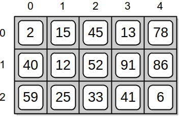
A one-dimensional array is commonly used to physically store arrays of higher dimensions. Consider a two-dimensional array divided into a table of rows and columns as illustrated in Figure 10.8.1.

Figure 10.8.1. The abstract view of a sample $3\times 5$ two-dimensional array.

To store the 2-D array in a single 1-D dynamic array, you must allocate space for the total number of elements in the 2-D array:

which results in the creation of the 1-D array

Array Storage

How can the individual elements of the table be stored in the one-dimensional structure while maintaining direct access to the individual table elements? There are two common approaches. The elements can be stored in row-major order or column-major order. Most high-level programming languages use row-major order, with FORTRAN being one of the few languages that uses column-major ordering to store and manage 2-D arrays.

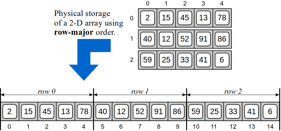
In row-major order, the individual rows are stored sequentially, one at a time, as illustrated in Figure 10.8.2. The first row of 5 elements are stored in the first 5 sequential elements of the 1-D array, the second row of 5 elements are stored in the next five sequential elements, and so forth.

Figure 10.8.2. Physical storage of a sample 2-D array (top) in a 1-D array using row-major order (bottom).

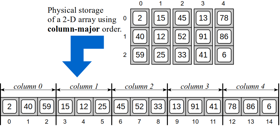
In column-major order, the 2-D array is stored sequentially, one entire column at a time, as illustrated in Figure 10.8.3. The first column of 3 elements are stored in the first 3 sequential elements of the 1-D array, followed by the 3 elements of the second column, and so on.

Figure 10.8.3. Physical storage of a sample 2-D array (top) in a 1-D array using column-major order (bottom).

For larger dimensions, a similar approach can be used. With a three-dimensional array, the individual tables can be stored contiguously using either row-major or column-major ordering. As the number of dimensions grow, all elements within a~single instance of each dimension are stored contiguously before the next instance. For example, given a four-dimensional array, which can be thought of as an array of boxes, all elements of an individual box (3-D array) are stored before the next box.

Index Computation

Since multi-dimensional arrays are created and managed by instructions in the programming language, accessing an individual element must also be handled by the language. When an individual element of a 2-D array is accessed, the compiler must include additional instructions to calculate the offset of the specific element within the 1-D array. Given a 2-D array of size $m\times n$ and using row-major ordering, an equation can be derived to compute this offset.

To derive the formula, consider the 2-D array illustrated in Figure 10.8.2 and observe the physical storage location within the 1-D array for the first element in several of the rows. Element $\mathit{\text{(0, 0)}}$ maps to position $\mathit{\text{0}}$ since it is the first element in both the abstract 2-D and physical 1-D arrays. The first entry of the second row $\mathit{\text{(1, 0)}}$ maps to position $n$ since it follows the first $n$ elements of the first row. Likewise, element $\mathit{\text{(2, 0)}}$ maps to position $\mathit{\text{2n}}$ since it follows the first $\mathit{\text{2n}}$ elements in the first two rows. We could continue in the same fashion through all of the rows, but you would soon notice the position for the first element of the $\mathit{\text{i}}$th row is $\mathit{\text{n * i}}$. Since the subscripts start from zero, the $\mathit{\text{i}}$ th subscript not only represents a specific row but also indicates the number of complete rows skipped to reach the $\mathit{\text{i}}$ th row.

Knowing the position of the first element of each row, the position for any element within a 2-D array can be determined. Given an element $\mathit{\text{(i, j)}}$ of a 2-D array, the storage location of that element in the 1-D array is computed as

$$\begin{array}{lcr}& {\text{index}}_2(i,j)=i*n+j& \end{array}$$

The column index, $j$, is not only the offset within the given row but also the number of elements that must be skipped in the $\mathit{\text{i}}$ th row to reach the $\mathit{\text{j}}$ th column. To see this formula in action, again consider the 2-D array from Figure 10.8.2 and assume we want to access element $\mathit{\text{(2, 3)}}$. Finding the target element within the 1-D array requires skipping over the first 2 complete rows of elements:

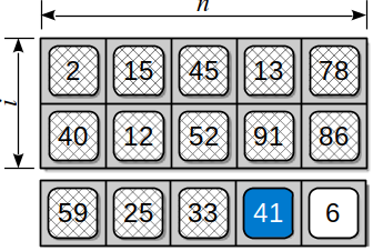
and the first 3 elements within row 2:

Plugging the indices into the equation from above results in an index position of 13, which corresponds to the position of element $\mathit{\text{(2, 3)}}$ within the 1-D array used to physically store the 2-D array.